Detecting Branches in Clusters

HDBSCAN* is often used to find subpopulations in exploratory data analysis workflows. Not only clusters themselves, but also their shape can represent meaningful subpopulations. For example, a Y-shaped cluster may represent an evolving process with two distinct end-states. Detecting these branches can reveal interesting patterns that are not captured by density-based clustering.

import numpy as np
import fast_hdbscan

import requests
from io import BytesIO
import seaborn as sns
import matplotlib.pyplot as plt

sns.set(rc={"figure.figsize":(8,8)})
data_request = requests.get(
    "https://github.com/scikit-learn-contrib/hdbscan/blob/master/notebooks/clusterable_data.npy?raw=true"
)
orig_data = np.load(BytesIO(data_request.content))

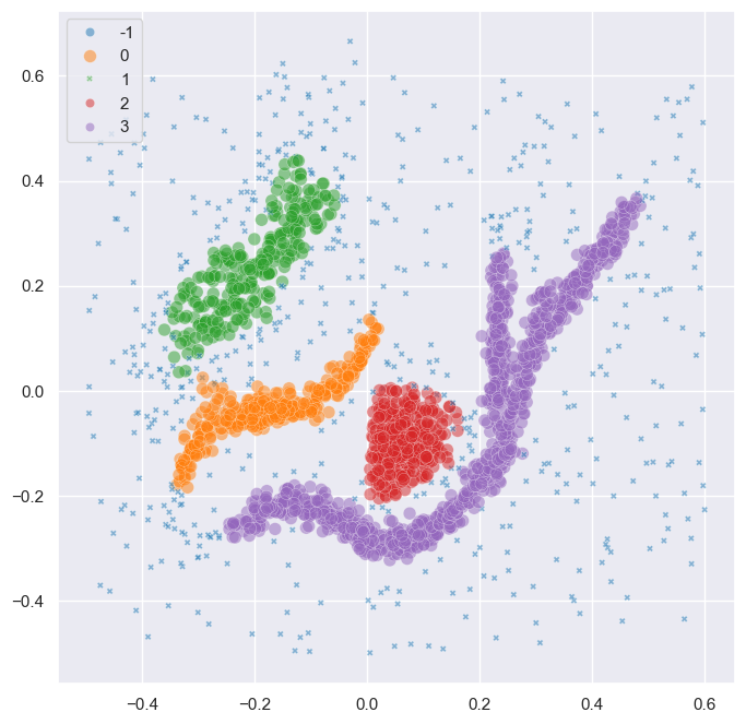
For example, HDBSCAN* finds 4 clusters in the datasets below, which does not inform us of the branching structure:

# merge three clusters into Y-shape
p0 = (0.13, -0.26)
p1 = (0.24, -0.12)
p2 = (0.32, 0.2)
segments = [
    np.column_stack(
        (np.linspace(p_start[0], p_end[0], 100),
         np.linspace(p_start[1], p_end[1], 100))
    )
    + np.random.normal(size=(100, 2), scale=0.01)
    for p_start, p_end in [(p0, p1), (p1, p2)]
]

data = np.concatenate((orig_data, *segments))
clusterer = fast_hdbscan.HDBSCAN(min_cluster_size=15).fit(data)
sns.scatterplot(
    x=data.T[0],
    y=data.T[1],
    hue=clusterer.labels_,
    style=clusterer.labels_ < 0,
    size=clusterer.labels_ < 0,
    palette="tab10",
    alpha=0.5,
)
plt.show()

Alternatively, HDBSCAN*’s leaf clusters provide more detail. They segment the points of different branches into distinct clusters. However, the partitioning and cluster hierarchy does not (necessarily) tell us how those clusters combine into a larger shape.

leaf_clusterer = fast_hdbscan.HDBSCAN(
    min_cluster_size=25, cluster_selection_method="leaf"
).fit(data)
sns.scatterplot(
    x=data.T[0],
    y=data.T[1],
    hue=leaf_clusterer.labels_,
    style=leaf_clusterer.labels_ < 0,
    size=leaf_clusterer.labels_ < 0,
    palette="tab10",
    alpha=0.5,
)
plt.show()

This is where the branch detection post-processing step comes into play. The functionality is described in detail by Bot et al. (please cite this paper when using this functionality). It operates on the detected clusters and extracts a branch-hierarchy analogous to HDBSCAN*’s condensed cluster hierarchy. The process is very similar to HDBSCAN* clustering, except that it operates on an in-cluster eccentricity rather than a density measure. Where peaks in a density profile correspond to clusters, the peaks in an eccentricity profile correspond to branches:

import matplotlib.tri as mtri

eccentricities = np.zeros(data.shape[0])
num_clusters = clusterer.labels_.max() + 1
for label in range(num_clusters):
    mask = clusterer.labels_ == label
    centroid = np.average(
        data[mask],
        weights=clusterer.probabilities_[mask],
        axis=0,
    )
    eccentricities[mask] = np.linalg.norm(data[mask] - centroid, axis=1)

fig = plt.figure()
tri = mtri.Triangulation(data[:, 0], data[:, 1])
ax = fig.add_subplot(1, 1, 1, projection="3d", computed_zorder=False)
ax.view_init(elev=45, azim=-100)
ax.scatter(
    data.T[0],
    data.T[1],
    np.repeat(eccentricities.min(), data.shape[0]),
    s=2,
    edgecolor="none",
    linewidth=0,
)
ax.tricontour(tri, eccentricities, levels=np.linspace(0, eccentricities.max(), 15))
zlim = ax.get_zlim()
ax.set_box_aspect(aspect=(3, 3, 1))

Using the branch detection functionality is fairly straightforward. Using fast_hdbscan one can simply configure the BranchDetector class and fit it with the fast_hdbscan.HDBSCAN object. By default BranchDetector uses the values of the given HDBSCAN object for the parameters they share.

The resulting partitioning reflects subgroups for clusters and their branches:

branch_detector = fast_hdbscan.BranchDetector().fit(clusterer)
sns.scatterplot(
    x=data.T[0],
    y=data.T[1],
    hue=branch_detector.labels_,
    style=branch_detector.labels_ < 0,
    size=branch_detector.labels_ < 0,
    palette="tab10",
    alpha=0.5,
)
plt.show()

The centers of clusters get a non-noise label different from the branches in the cluster. This behavior can be changed by setting the propagate_labels=True parameter or by calling propagated_labels() after fitting.

labels, _ = branch_detector.propagated_labels()
sns.scatterplot(
    x=data.T[0],
    y=data.T[1],
    hue=labels,
    style=labels < 0,
    size=labels < 0,
    palette="tab10",
    alpha=0.5,
)
plt.show()

Parameter selection

The BranchDetector’s main parameters are very similar to HDBSCAN*. Most guidelines for tuning HDBSCAN* also apply to the branch detector:

• min_cluster_size configures how many points branches need to contain. Values around 10 to 25 points tend to work well. Lower values are useful when looking for smaller structures. Higher values can be used to suppress noise if present.

• max_cluster_size. Branches with more than the specified number of points are skipped, selecting their descendants in the hierarchy instead.

• cluster_selection_method. The leaf and Excess of Mass (EOM) strategies are used to select branches from the condensed hierarchies. By default, branches are only reflected in the final labelling for clusters that have 3 or more branches (at least one bifurcation).

• cluster_selection_epsilon can be used to suppress branches that merge at low eccentricity values (y-value in the condensed hierarchy plot).

• cluster_selection_persistence can be used to suppress branches with a short eccentricity range (y-range in the condensed hierarchy plot).

• allow_single_cluster. When enabled, clusters with bifurcations will be given a single label if the root segment contains most eccentricity mass (i.e., branches already merge far from the center and most points are central).

One parameter is unique to the BranchDetector class:

• label_sides_as_branches determines whether the sides of an elongated cluster without bifurcations (l-shape) are represented as distinct subgroups. By default a cluster needs to have one bifurcation (Y-shape) before the detected branches are represented in the final labelling.

Unlike the hdbscan version, fast_hdbscan’s BranchDetector does not support the branch_detection_method parameter. This implementation will always use a "core" graph to determine which points are connected within a cluster. A "core" graph combines nearest neighbors and the minimum spanning tree of a cluster. It contains all connectivity within the points’ core distances and forms a single connected component per cluster.

Useful attributes

The BranchDetector class contains several useful attributes for exploring datasets.

Branch hierarchy

Branch hierarchies reflect the tree-shape of clusters. Like the cluster hierarchy, branch hierarchies can be used to interpret which branches exist. In addition, they reflect how far apart branches merge into the cluster.

branch_detector.condensed_trees_[3].plot(select_clusters=True, selection_palette=['C5', 'C6', 'C7'])
plt.ylabel("Eccentricity")
plt.title(f"Branches in cluster {3}")
plt.show()

The length of the branches also says something about the compactness / elongatedness of clusters. For example, the branch hierarchy for the orange ~-shaped cluster is quite different from the same hierarchy for the central o-shaped cluster.

plt.figure(figsize=(6, 3))
plt.subplot(1, 2, 1)
branch_detector.condensed_trees_[2].plot(colorbar=False)
plt.ylim([0.3, 0])
plt.ylabel("Eccentricity")
plt.title(f"Cluster {2} (spherical)")

plt.subplot(1, 2, 2)
branch_detector.condensed_trees_[1].plot(colorbar=False)
plt.ylim([0.3, 0])
plt.ylabel("Eccentricity")
plt.title(f"Cluster {1} (elongated)")
plt.show()

Cluster approximation graphs

Branches are detected using a graph that approximates the connectivity within a cluster. These graphs are available in the cluster_approximation_graph_ property and can be used to visualize data and the branch-detection process. The plotting function is based on the networkx API and uses networkx functionality to compute a layout if positions are not provided. Using UMAP to compute positions can be faster and more expressive. Several helper functions for exporting to numpy, pandas, and networkx are available.

For example, a figure with points coloured by the final labelling:

g = branch_detector.approximation_graph_
g.plot(positions=data, node_size=5, edge_width=0.2, edge_alpha=0.2)
plt.show()

Or, a figure with the edges coloured by centrality:

g.plot(
    positions=data,
    node_alpha=0,
    edge_color="centrality",
    edge_cmap="turbo",
    edge_width=0.2,
    edge_alpha=0.2,
    edge_vmax=100,
)
plt.show()

Detect branches in other clusters

It is possible to evaluate the BranchDetector class with non-HDBSCAN clusters through the optional arguments of its .fit() method. In the example below, two clusters are merged manually, resulting in a different branching structure. This functionality can be used to look for branches in, f.i., DBSCAN labels.

# Valid option
custom_labels = clusterer.labels_.copy()
custom_labels[clusterer.labels_ == 3] = 2
branch_detector.fit(clusterer, custom_labels)

sns.scatterplot(
    x=data.T[0],
    y=data.T[1],
    hue=branch_detector.labels_,
    style=branch_detector.labels_ < 0,
    size=branch_detector.labels_ < 0,
    palette="tab10",
    alpha=0.5,
)
plt.show()

Custom clusters only work if they are within-cluster-path-connected in HDBSCAN’s minimum spanning tree (MST). In other words, the MST edges between all points in the cluster must form a single connected component. Custom clusters that break this condition return the MST connected component labels instead of branches, without looking for branches!!

# Invalid labels cannot find branches!
custom_labels = clusterer.labels_.copy()
custom_labels[clusterer.labels_ == 3] = 0
branch_detector.fit(clusterer, custom_labels)

sns.scatterplot(
    x=data.T[0],
    y=data.T[1],
    hue=branch_detector.labels_,
    style=branch_detector.labels_ < 0,
    size=branch_detector.labels_ < 0,
    palette="tab10",
    alpha=0.5,
)
plt.show()

Citing

If you used the branch-detection functionality in this library please cite our PeerJ paper:

D.M. Bot, J. Peeters, J. Liesenborgs, J. Aerts. FLASC: a flare-sensitive clustering algorithm. PeerJ Computer Science, Volume 11, e2792, 2025. https://doi.org/10.7717/peerj-cs.2792.

@article{bot2025flasc,
    title   = {{FLASC: a flare-sensitive clustering algorithm}},
    author  = {Bot, Dani{\"{e}}l M. and Peeters, Jannes and Liesenborgs, Jori and Aerts, Jan},
    year    = {2025},
    month   = {apr},
    journal = {PeerJ Comput. Sci.},
    volume  = {11},
    pages   = {e2792},
    issn    = {2376-5992},
    doi     = {10.7717/peerj-cs.2792},
    url     = {https://peerj.com/articles/cs-2792},
}