For Developers

This notebook outlines design choices made in fast_hdbscan and is intended for developers who want to build upon (parts of) fast_hdbscan in their projects (for example, see the fast_hbcc repository).

import seaborn as sns
import matplotlib.pyplot as plt
from sklearn.datasets import make_blobs

sns.set(rc={"figure.figsize":(8,8)})

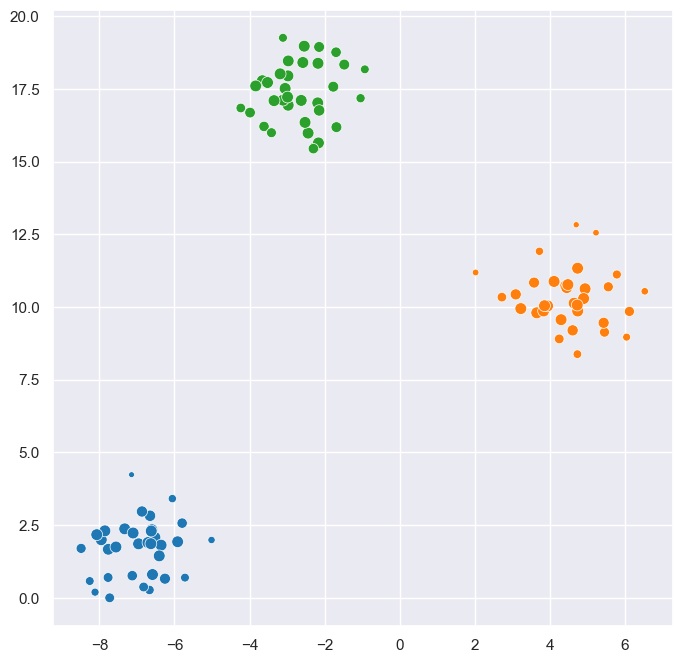
X, y = make_blobs(centers=3, random_state=42)
X[:, 1] -= X[:, 1].min()

Main API

fast_hdbscan exposes two scikit-learn-style cluster estimators (HDBSCAN and BranchDetector) and their respective function versions (fast_hdbscan(), find_branch_sub_clusters()) as its main API. This API is demonstrated in the basic_usage and detecting_branches pages.

Building Blocks

The HDBSCAN algorithm consists of two stages, that are each implemented as a single function: (1) computing the minimum spanning tree and (2) extracting clusters from a minimum spanning tree. Separating the algorithm into these stages enables re-use of the cluster extraction functionality on different minimum spanning trees. For example, to use different local density estimates or different minimum spanning trees construction algorithms.

1. fast_hdbscan.hdbscan.compute_minimum_spanning_tree computes a Euclidean mutual reachability distance minimum spanning tree. It takes the data, optional sample weights, and a value for min_samples as input. Aside from the minimum spanning tree edges, the function also returns the min_samples-nearest neighbors and the points’ core distances:

from fast_hdbscan.hdbscan import compute_minimum_spanning_tree

spanning_tree, neighbors, core_distances = compute_minimum_spanning_tree(
    X, min_samples=5, sample_weights=None
)

# Core distance colored points
sns.scatterplot(x=X[:, 0], y=X[:, 1], hue=core_distances, palette="viridis")

# Dotted neighbor edges
for row, children in enumerate(neighbors):
    for child in children:
        plt.plot(
            [X[row, 0], X[child, 0]],
            [X[row, 1], X[child, 1]],
            c="black",
            linestyle=":",
            alpha=0.5,
        )

# Solid minimum spanning tree edges
for parent, child in spanning_tree[:, :2].astype(int):
    plt.plot(
        [X[parent, 0], X[child, 0]], [X[parent, 1], X[child, 1]], c="black", alpha=0.5
    )

plt.show()

2. fast_hdbscan.hdbscan.clusters_from_spanning_tree extracts clusters from a minimum spanning tree. It takes the minimum spanning tree as input, together with the parameters that control cluster selection. It outputs the resulting cluster labels, membership strengths, the single linkage tree, the condensed cluster tree, and the sorted minimum spanning tree edges.

from fast_hdbscan.hdbscan import clusters_from_spanning_tree

labels, probability, linkage_tree, condensed_tree, sorted_mst = (
    clusters_from_spanning_tree(
        spanning_tree, min_cluster_size=15, cluster_selection_method="eom"
    )
)

sns.scatterplot(
    x=X[:, 0], y=X[:, 1], hue=labels, size=probability, palette="tab10", legend=False
)
plt.show()

The branch-detection functionality is also divided into two parts, implemented in the core_graph and sub_clusters modules. These modules are implemented independently of the branch detection functionality. Where the branch detector uses an eccentricity lens (i.e., a value for each data point), these modules can be used with any (preferably fairly smooth) lens.

Broadly speaking, the core_graph module deals with finding clusters in a lens dimension while restricting connectivity to the minimum spanning tree and nearest neighbor edges. The sub_clusters module deals with finding such lensed-clusters within each detected HDBSCAN cluster.

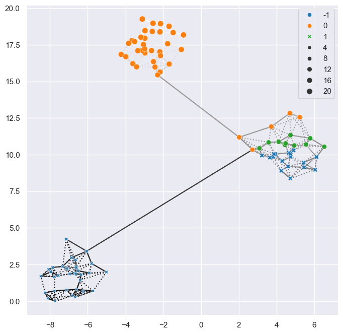
3. fast_hdbscan.core_graph.core_graph_clusters extracts lensed-clusters restricted to core graph connectivity. First, it creates a core graph with edges weighted by the maximum lens value of the points they connect. Second, it extract a minimum spanning tree using the lens weights. Finally, it calls clusters_from_spanning_tree to extract clusters from that minimum spanning tree. The output contains everything from clusters_from_spanning_tree and the constructed core graph in sparse CSR format. Should the function fail to create a minimum spanning tree because the core graph contains multiple connected components, then the component labels and empty linkage and core trees are returned.

from fast_hdbscan.core_graph import core_graph_clusters

# use 1 / y as lens for demonstration
lens = 1 / (X[:, 1] + 1)

labels, probability, linkage_tree, condensed_tree, sorted_mst, graph = (
    core_graph_clusters(
        lens,
        neighbors,
        core_distances,
        spanning_tree,
        min_cluster_size=10,
        cluster_selection_method="eom",
    )
)

# label-colored, lens-sized points
sns.scatterplot(
    x=X[:, 0],
    y=X[:, 1],
    hue=labels,
    style=labels < 0,
    size=1 / lens,
    palette="tab10",
    zorder=100,
)

# dotted lens-colored core_graph edges
for parent, (start, end) in enumerate(zip(graph.indptr, graph.indptr[1:])):
    for child, weight in zip(graph.indices[start:end], graph.weights[start:end]):
        plt.plot(*X[[parent, child]].T, c=f"{(1 / weight) / 20}", linestyle=":")

# solid lens-colored mst edges
for parent, child, weight in sorted_mst:
    parent = int(parent)
    child = int(child)
    plt.plot(*X[[parent, child]].T, c=f"{(1 / weight) / 20}")

plt.show()

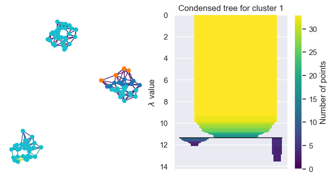
4. fast_hdbscan.sub_clusters.SubClusterDetector is the general base class for BranchDetector. It takes either an array with lens values at construction, or a callback to compute lens values within a cluster at .fit(clusterer) and computes lensed clusters within each HDBSCAN detected cluster. The class also exposes properties for the minimum spanning trees, single linkage trees, condensed cluster trees, and approximation graph.

There are two use cases for the SubClusterDetector. Either directly with a pre-computed lens:

from fast_hdbscan import HDBSCAN
from fast_hdbscan.sub_clusters import SubClusterDetector

clusterer = HDBSCAN(min_cluster_size=5).fit(X)
detector = SubClusterDetector(lens_values=lens, min_cluster_size=2).fit(clusterer)

plt.figure(figsize=(8, 4))
plt.subplot(1, 2, 1)
detector.approximation_graph_.plot(
    positions=X, node_size=40, node_color="sub_cluster_label", edge_color="lens_value"
)
plt.subplot(1, 2, 2)
detector.condensed_trees_[1].plot()
plt.title("Condensed tree for cluster 1")
plt.show()

Or as a base class with a lens callback. This approach can deal with parameters on the lens function and provide aliases that make sense for the lens function.

from typing import Literal


def make_y_callback(offset):
    """Takes the detector-specific parameters and returns a callback function."""

    def y_callback(
        data, cluster_probability, neighbors, core_distances, min_spanning_tree, points
    ):
        """
        Parameters
        ----------
        data : np.ndarray
            Full clean data array.
        cluster_probability : np.ndarray
            Full clean array of cluster probabilities.
        neighbors : np.ndarray
            Within cluster neighbor array, with ids relabelled to 0, ..., num_points_in_cluster.
        core_distances : np.ndarray
            Within cluster core distance array.
        points : np.ndarray
            List of clean data point ids for the current cluster.
        """
        return 1 / (data[points, 1] + offset)

    return y_callback


class YDetector(SubClusterDetector):
    def __init__(
        self,
        y_offset: float = 1,  # detector-specific parameter
        min_cluster_size: int | None = None,
        max_cluster_size: int | None = None,
        allow_single_cluster: bool | None = None,
        cluster_selection_method: Literal["eom", "leaf"] | None = None,
        cluster_selection_epsilon: float = 0.0,
        cluster_selection_persistence: float = 0.0,
        propagate_labels: bool = False,
    ):
        super().__init__(
            min_cluster_size=min_cluster_size,
            max_cluster_size=max_cluster_size,
            allow_single_cluster=allow_single_cluster,
            cluster_selection_method=cluster_selection_method,
            cluster_selection_epsilon=cluster_selection_epsilon,
            cluster_selection_persistence=cluster_selection_persistence,
            propagate_labels=propagate_labels,
        )
        self.y_offset = y_offset

    def fit(self, clusterer, labels=None, probabilities=None, sample_weight=None):
        super().fit(
            clusterer,
            labels,
            probabilities,
            sample_weight,
            make_y_callback(self.y_offset),
        )
        self.y_values_ = self.lens_values_  # add y_values_ alias for lens_values_
        return self

    # Override to specify lens and sub_cluster names.
    @property
    def approximation_graph_(self):
        """See :class:`~hdbscan.plots.ApproximationGraph` for documentation."""
        return super()._make_approximation_graph(
            lens_name="y_value", sub_cluster_name="y_cluster"
        )

detector = YDetector(min_cluster_size=2).fit(clusterer)

plt.figure(figsize=(8, 4))
plt.subplot(1, 2, 1)
detector.approximation_graph_.plot(
    positions=X, node_size=40, node_color="y_cluster_label", edge_color="y_value"
)
plt.subplot(1, 2, 2)
detector.condensed_trees_[1].plot()
plt.title("Condensed tree for cluster 1")
plt.show()