Multi-Resolution Clustering with PLSCAN

One of the trickiest aspects of using HDBSCAN is choosing the min_cluster_size parameter. Different values can reveal very different structure in your data, and it’s not always clear which resolution is the “right” one. fast_hdbscan provides the PLSCAN class which automates this process entirely. PLSCAN finds all meaningful clustering resolutions in your data, ranks them by a persistence score, and returns the best one – along with all the other layers for you to explore. It implements the algorithm described in Persistent Multiscale Density-based Clustering. Let’s load some libraries and grab some data to see it in action:

import numpy as np
import fast_hdbscan

import requests
from io import BytesIO
import seaborn as sns
import matplotlib.pyplot as plt
from sklearn.datasets import make_blobs

sns.set(rc={"figure.figsize":(8,8)})
data_request = requests.get(
    "https://github.com/scikit-learn-contrib/hdbscan/blob/master/notebooks/clusterable_data.npy?raw=true"
)
data = np.load(BytesIO(data_request.content))

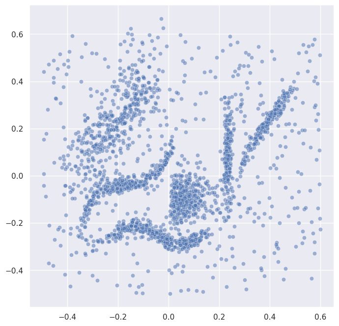
This is the same dataset used in the basic usage notebook. Before we cluster, let’s plot it so we can see what we’re working with:

sns.scatterplot(x=data.T[0], y=data.T[1], alpha=0.5)

<Axes: >

The resolution problem

Let’s illustrate why choosing min_cluster_size can be tricky. We’ll run HDBSCAN with two very different values and see what happens:

labels_fine = fast_hdbscan.HDBSCAN(min_cluster_size=5).fit_predict(data)
labels_coarse = fast_hdbscan.HDBSCAN(min_cluster_size=50).fit_predict(data)

fig, axes = plt.subplots(1, 2, figsize=(16, 8))
for ax, labels, title in zip(
    axes,
    [labels_fine, labels_coarse],
    ["min_cluster_size=15", "min_cluster_size=100"],
):
    sns.scatterplot(
        x=data.T[0], y=data.T[1], alpha=0.5,
        hue=labels, style=labels < 0, size=labels < 0,
        palette="tab10", legend=False, ax=ax,
    )
    ax.set_title(title)

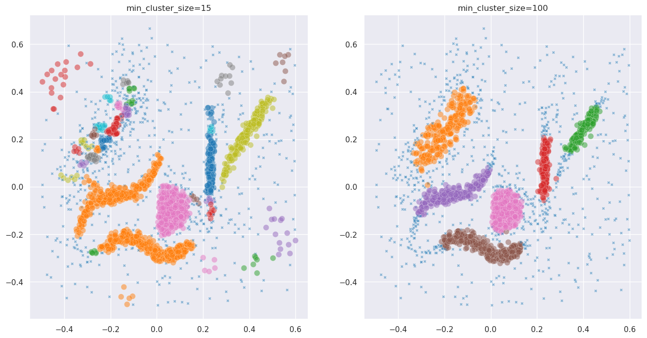
Different values of min_cluster_size reveal different structure. Which is the right answer? It depends on what you’re looking for – and choosing can feel like guesswork. PLSCAN finds all meaningful resolutions automatically, with almost no parameter tuning.

Basic PLSCAN usage

Using PLSCAN is as simple as using HDBSCAN. You create a PLSCAN object and call fit_predict on your data. The default parameters work well for most datasets:

clusterer = fast_hdbscan.PLSCAN()
labels = clusterer.fit_predict(data)

The labels_ attribute gives you the best clustering – the layer with the highest persistence score. Let’s plot it:

sns.scatterplot(
    x=data.T[0], y=data.T[1], alpha=0.5,
    hue=clusterer.labels_, style=clusterer.labels_ < 0, size=clusterer.labels_ < 0,
    palette="tab10", legend=False,
)

<Axes: >

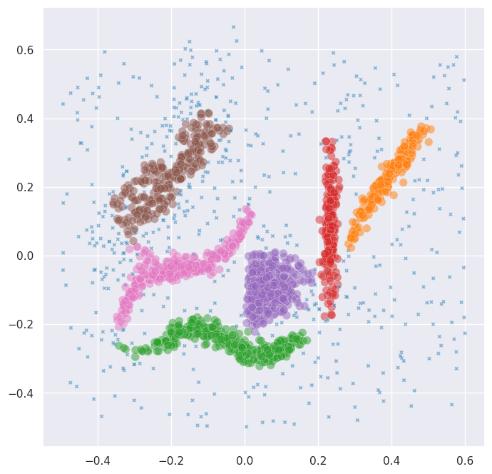
With no parameter tuning at all, PLSCAN found a good clustering of the data.

Exploring the layers

PLSCAN doesn’t just give you one clustering – it finds all meaningful resolutions. These are stored in the cluster_layers_ attribute. Each layer is an array of cluster labels at a different resolution. Let’s see how many layers PLSCAN found and what their persistence scores are:

print(f"Number of layers: {len(clusterer.cluster_layers_)}")
print(f"Persistence scores: {clusterer.layer_persistence_scores_}")

Number of layers: 4
Persistence scores: [0.0, np.float32(752.7444), np.float32(1556.6232), np.float32(1452.8157)]

Let’s plot each layer so we can see what resolutions PLSCAN identified:

n_layers = len(clusterer.cluster_layers_)
fig, axes = plt.subplots(1, n_layers, figsize=(8 * n_layers, 8))
if n_layers == 1:
    axes = [axes]
for i, (ax, layer_labels) in enumerate(zip(axes, clusterer.cluster_layers_)):
    n_clusters = len(set(layer_labels[layer_labels >= 0]))
    sns.scatterplot(
        x=data.T[0], y=data.T[1], alpha=0.5,
        hue=layer_labels, style=layer_labels < 0, size=layer_labels < 0,
        palette="tab10", legend=False, ax=ax,
    )
    ax.set_title(f"Layer {i}: {n_clusters} clusters (persistence: {clusterer.layer_persistence_scores_[i]:.2f})")

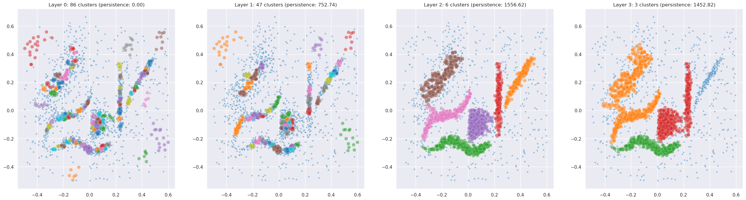
For this particular dataset PLSCAN may find only one or two meaningful resolutions. That’s itself informative – it tells you there’s really only one good scale of clustering in this data. To see PLSCAN really shine, we need data with genuine multi-scale structure.

Multi-scale synthetic data

Let’s build a dataset with nested structure: a few large macro-clusters, each of which contains tighter sub-clusters inside it. This kind of hierarchical structure is common in real-world data – think of species within genera, or neighbourhoods within cities.

rng = np.random.RandomState(42)

# Macro-cluster centers, spread far apart
macro_centers = np.array([[0, 0], [12, 0], [6, 10]])

# Within each macro-cluster, place 2-3 sub-clusters
sub_offsets = [
    [[-1.5, -1], [1.5, -1], [0, 1.5]],   # 3 sub-clusters in macro 0
    [[-1.5, 0], [1.5, 0]],                 # 2 sub-clusters in macro 1
    [[-1, -1], [1, -1], [0, 1.5]],         # 3 sub-clusters in macro 2
]
sub_sizes = [
    [150, 150, 100],
    [200, 200],
    [150, 150, 100],
]

nested_data = []
for macro_center, offsets, sizes in zip(macro_centers, sub_offsets, sub_sizes):
    for offset, n in zip(offsets, sizes):
        center = macro_center + np.array(offset)
        nested_data.append(rng.normal(center, 0.5, size=(n, 2)))

nested_data = np.vstack(nested_data)

sns.scatterplot(x=nested_data.T[0], y=nested_data.T[1], alpha=0.5)

<Axes: >

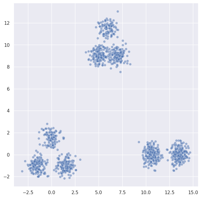
You can see three macro-clusters, and if you look closely each one contains smaller sub-clusters. Let’s see what PLSCAN makes of this:

PLSCAN on nested data

nested_clusterer = fast_hdbscan.PLSCAN()
nested_labels = nested_clusterer.fit_predict(nested_data)

print(f"Number of layers: {len(nested_clusterer.cluster_layers_)}")
print(f"Persistence scores: {nested_clusterer.layer_persistence_scores_}")

Number of layers: 4
Persistence scores: [0.0, np.float32(387.75885), np.float32(1050.1278), np.float32(1200.0)]

n_layers = len(nested_clusterer.cluster_layers_)
fig, axes = plt.subplots(1, n_layers, figsize=(8 * n_layers, 8))
if n_layers == 1:
    axes = [axes]
for i, (ax, layer_labels) in enumerate(zip(axes, nested_clusterer.cluster_layers_)):
    n_clusters = len(set(layer_labels[layer_labels >= 0]))
    sns.scatterplot(
        x=nested_data.T[0], y=nested_data.T[1], alpha=0.5,
        hue=layer_labels, style=layer_labels < 0, size=layer_labels < 0,
        palette="tab10", legend=False, ax=ax,
    )
    ax.set_title(f"Layer {i}: {n_clusters} clusters (persistence: {nested_clusterer.layer_persistence_scores_[i]:.2f})")

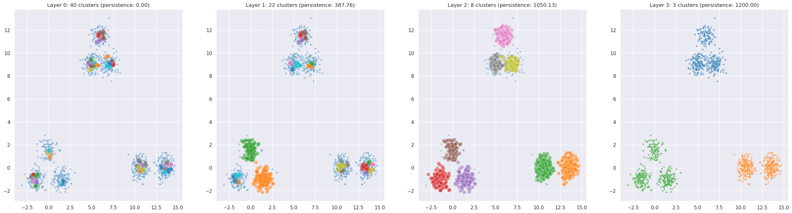
Now we can see PLSCAN in its element. It automatically found both the coarse structure (the macro-clusters) and the fine structure (the sub-clusters) without any manual parameter tuning. The persistence scores tell you how robust each resolution is.

Persistence barcode

PLSCAN selects its layers by looking for peaks in a persistence score – a function that measures how robust the clustering is at each possible resolution. We can plot this to see where the meaningful resolutions are:

fig, ax = plt.subplots(figsize=(12, 4))
ax.plot(
    np.column_stack(
        (nested_clusterer.min_cluster_sizes_[:-1], nested_clusterer.min_cluster_sizes_[1:])
    ).reshape(-1),
    np.repeat(nested_clusterer.total_persistence_[:-1], 2),
)
ax.set_xlabel("Cluster size threshold")
ax.set_ylabel("Total persistence")
ax.set_title("Persistence score")
plt.tight_layout()

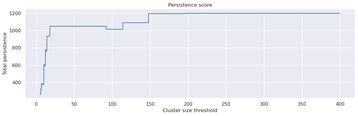
The peaks in this plot correspond to cluster resolutions that are particularly robust. PLSCAN automatically identifies these peaks and extracts a clustering at each one. The height of the peak corresponds to the persistence score – higher peaks mean more robust clusterings.

Cluster tree

When you have multiple layers, it’s natural to ask how the clusters relate across resolutions. The cluster_tree_ attribute provides this mapping. It is a dictionary where each key is a (layer, cluster_id) tuple representing a parent cluster, and the value is a list of (layer, cluster_id) tuples for its children at finer resolutions:

for parent, children in nested_clusterer.cluster_tree_.items():
    print(f"Layer {parent[0]}, Cluster {parent[1]} -> {[(f'Layer {c[0]}, Cluster {c[1]}') for c in children]}")

Layer 1, Cluster 0 -> ['Layer 0, Cluster 28', 'Layer 0, Cluster 29']
Layer 1, Cluster 1 -> ['Layer 0, Cluster 8', 'Layer 0, Cluster 0', 'Layer 0, Cluster 7']
Layer 1, Cluster 2 -> ['Layer 0, Cluster 2']
Layer 1, Cluster 3 -> ['Layer 0, Cluster 3']
Layer 1, Cluster 4 -> ['Layer 0, Cluster 4']
Layer 1, Cluster 5 -> ['Layer 0, Cluster 5']
Layer 1, Cluster 6 -> ['Layer 0, Cluster 6']
Layer 1, Cluster 7 -> ['Layer 0, Cluster 9']
Layer 1, Cluster 8 -> ['Layer 0, Cluster 11', 'Layer 0, Cluster 12']
Layer 1, Cluster 9 -> ['Layer 0, Cluster 15', 'Layer 0, Cluster 14']
Layer 1, Cluster 10 -> ['Layer 0, Cluster 13']
Layer 1, Cluster 11 -> ['Layer 0, Cluster 16']
Layer 1, Cluster 12 -> ['Layer 0, Cluster 25', 'Layer 0, Cluster 26', 'Layer 0, Cluster 19']
Layer 1, Cluster 13 -> ['Layer 0, Cluster 18']
Layer 1, Cluster 14 -> ['Layer 0, Cluster 20']
Layer 1, Cluster 15 -> ['Layer 0, Cluster 23']
Layer 1, Cluster 16 -> ['Layer 0, Cluster 24']
Layer 1, Cluster 17 -> ['Layer 0, Cluster 33', 'Layer 0, Cluster 35', 'Layer 0, Cluster 37', 'Layer 0, Cluster 36']
Layer 1, Cluster 18 -> ['Layer 0, Cluster 32', 'Layer 0, Cluster 30', 'Layer 0, Cluster 31']
Layer 1, Cluster 19 -> ['Layer 0, Cluster 27']
Layer 1, Cluster 20 -> ['Layer 0, Cluster 38']
Layer 1, Cluster 21 -> ['Layer 0, Cluster 39']
Layer 2, Cluster 0 -> ['Layer 1, Cluster 12', 'Layer 1, Cluster 5', 'Layer 1, Cluster 13', 'Layer 1, Cluster 7', 'Layer 1, Cluster 11']
Layer 2, Cluster 1 -> ['Layer 1, Cluster 17', 'Layer 1, Cluster 16', 'Layer 1, Cluster 6', 'Layer 1, Cluster 14', 'Layer 0, Cluster 17']
Layer 2, Cluster 2 -> ['Layer 1, Cluster 8', 'Layer 1, Cluster 9', 'Layer 1, Cluster 10', 'Layer 0, Cluster 1']
Layer 2, Cluster 3 -> ['Layer 1, Cluster 0']
Layer 2, Cluster 4 -> ['Layer 1, Cluster 1']
Layer 2, Cluster 5 -> ['Layer 1, Cluster 2', 'Layer 1, Cluster 4', 'Layer 1, Cluster 3']
Layer 2, Cluster 6 -> ['Layer 1, Cluster 19', 'Layer 1, Cluster 15', 'Layer 1, Cluster 18', 'Layer 0, Cluster 21']
Layer 2, Cluster 7 -> ['Layer 1, Cluster 21', 'Layer 1, Cluster 20', 'Layer 0, Cluster 22', 'Layer 0, Cluster 34', 'Layer 0, Cluster 10']
Layer 3, Cluster 0 -> ['Layer 2, Cluster 6', 'Layer 2, Cluster 7', 'Layer 2, Cluster 5']
Layer 3, Cluster 1 -> ['Layer 2, Cluster 0', 'Layer 2, Cluster 1']
Layer 3, Cluster 2 -> ['Layer 2, Cluster 2', 'Layer 2, Cluster 3', 'Layer 2, Cluster 4']
Layer 4, Cluster 0 -> ['Layer 3, Cluster 0', 'Layer 3, Cluster 1', 'Layer 3, Cluster 2']

This tells you exactly which coarse-grained clusters split into which fine-grained sub-clusters, giving you a hierarchical view of the structure in your data.

Parameter tuning

While PLSCAN works well with default parameters, there are a few knobs you can turn:

• base_min_cluster_size controls the finest resolution explored. Smaller values allow PLSCAN to find smaller clusters. The default of 10 works well for most datasets.

• base_n_clusters is an alternative to base_min_cluster_size. If set, PLSCAN will binary search for a min_cluster_size that produces approximately this many clusters in the base layer.

• max_layers caps how many layers PLSCAN will return. The default of 10 is generous; most datasets have far fewer meaningful resolutions.

• layer_similarity_threshold controls how diverse the returned layers need to be. Higher values mean fewer, more distinct layers; lower values allow more similar layers through. The default of 0.2 is a good starting point.

• min_samples plays the same role as in HDBSCAN – it controls the density estimation. If not set, it defaults to min_samples=5.

Let’s see the effect of layer_similarity_threshold on our nested data:

for threshold in [0.0, 0.25, 0.5]:
    plscan = fast_hdbscan.PLSCAN(layer_similarity_threshold=threshold)
    plscan.fit(nested_data)
    n_layers = len(plscan.cluster_layers_)
    n_clusters_per_layer = [len(set(l[l >= 0])) for l in plscan.cluster_layers_]
    print(f"threshold={threshold}: {n_layers} layers with {n_clusters_per_layer} clusters each")

threshold=0.0: 3 layers with [40, 8, 3] clusters each
threshold=0.25: 4 layers with [40, 15, 8, 3] clusters each
threshold=0.5: 6 layers with [40, 22, 15, 11, 8, 3] clusters each

Higher thresholds allow more similar layers through, so you tend to get more layers. Lower thresholds are more selective, keeping only the most distinct resolutions.

Citing

If you use PLSCAN in your work please cite the paper:

@article{plscan2024,
    title   = {{Persistent Multiscale Density-based Clustering}},
    year    = {2024},
    eprint  = {2512.16558},
    archivePrefix = {arXiv},
    primaryClass  = {cs.LG},
    url     = {https://arxiv.org/abs/2512.16558},
}